################################### TODO ###################################
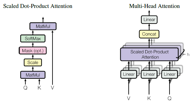
# Implement Multi-head attention described above.
############################################################################
class MultiHeadAttention(nn.Module):
def __init__(self, embed_dim, n_heads, attn_drop_rate):
"""
Parameters:
input_dim: The input dimension.
embed_dim: The embedding dimension of the model
n_heads: Number of attention heads
attn_drop_rate: Dropout rate for attention weights (Q K^T)
"""
super().__init__()
self.embed_dim = embed_dim
self.n_heads = n_heads
self.head_dim = embed_dim // n_heads
self.attn_drop_rate = attn_drop_rate
# TODO: Add learnable parameters for computing query, key, and value using nn.Linear.
# Store all weight matrices W^Q, W^K, W^V 1...h together for efficiency.
self.qkv_proj = nn.Linear(self.embed_dim, 3*self.embed_dim)
# TODO: Add learnable parameters W^O using nn.Linear.
self.o_proj = nn.Linear(self.embed_dim, self.embed_dim)
self._reset_parameters()
def _reset_parameters(self):
# Original Transformer initialization, see PyTorch documentation
nn.init.xavier_uniform_(self.qkv_proj.weight)
self.qkv_proj.bias.data.fill_(0)
nn.init.xavier_uniform_(self.o_proj.weight)
self.o_proj.bias.data.fill_(0)
def forward(self, embedding, mask):
"""
Inputs:
embedding: Input embedding with shape (batch size, sequence length, embedding dimension)
mask: Mask specifying padding tokens with shape (batch_size, sequence length)
Value for tokens that should be masked out is 1 and 0 otherwise.
Outputs:
Attended values
"""
# TODO: get batch_size, seq_length, embed_dim.
batch_size, seq_length, embed_dim = embedding.size()
# TODO: Compute queries, keys, and values (keep continguous for now).
qkv = self.qkv_proj(embedding)
# TODO: Separate Q, K, V from linear output, give each shape [batch, num_head, seq_len, head_dim] (may require transposing/permuting dimensions)
qkv = qkv.reshape(batch_size, seq_length, self.n_heads, 3*self.head_dim)
qkv = qkv.permute(0, 2, 1, 3)
q, k, v = qkv.chunk(3, dim=-1)
# TODO: Determine value outputs, with shape [batch, seq_len, num_head, head_dim]. (hint: use scaled_dot_product())
if mask is None:
values, attention = scaled_dot_product(q, k, v, attn_drop_rate=self.attn_drop_rate)
else:
values, attention = scaled_dot_product(q, k, v, attn_drop_rate=self.attn_drop_rate,
mask=mask.reshape([batch_size, 1, 1, seq_length]).repeat(1, self.n_heads, 1, 1))
# TODO: Linearly project attention outputs w/ W^O.
# The final dimensionality should match that of the inputs.
values = values.permute(0, 2, 1, 3) # [Batch, SeqLen, Head, Dims]
values = values.reshape(batch_size, seq_length, embed_dim)
attended_embeds = self.o_proj(values)
return attended_embeds